by Stephen Fegan

Overview

• AGN analysis is much the same as for other source types, but some tasks more relevant, so certain “problems” more common
• Light curve calculation - tutorial / problems
• Variability testing - 1FGL and 2FGL methods
• Absolute “goodness 0f fit” measure in spectral modeling
• Flux / Index correlations

Light curve tutorial

• LC creation: Regular / adaptive binning with LA, AP method, and Bayesian blocks (constant rate segments)
• Choice depends on Ur needs
• Flux v.s. Flux/Index LC

Regular flux calculation with likelihood

1. Perform a standard LA of full time period.
2. Determine what binning is reasonable.
   • Science goals and strength of source of interest.
   • Bins should not be much larger than $TS_{Tot} / 25$.
   • Affection of upper limits on the ayalysis.
   • Avoid periods close to being integer fractions of the orbital precessional period of $53.7$ days.
3. Prepare an ROI model for the time bins.
   • Freeze spectral shapes of all background sources.
   • Freeze all parameters of weak background sources - Will cause convergence problems. $TS_{Tot} / N_{bin} < 4$ or $9$.
   • For flux only LC, freeze spectral shape of source of interest.
4. Decide on criteria for upper limits.
   • $TS_i < 10$ or ${\Delta}F_i / F_i > 0.5$ (or $N_{predi}< 3$)
   • $95\%$ Bayesian UL when $TS_i < 1$
   • $95\%$ profile method otherwise. [$\delta = chi2inv(2*(0.95-0.5))/2 = 2.71/2$]¹
5. Divide data into bins (gtselect).
6. Run likelihood analysis on each.
7. Check each analysis for problems.
8. Compute upper limits where necessary.

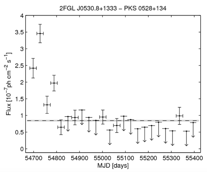
Example from 2FGL

Error-matrix problems in LCs

• The minimizer may not give proper error matrix in calculation of LC points.
• Usually the minimizer will converge, and the model parameters will be OK.
• But the errors can be VERY wrong.
• Hence a $\chi^2$ fit to a constant can be wrong.
• This seems to be related to parameters that are not properly constrained (and hence hit limits).

A sample LAT LC

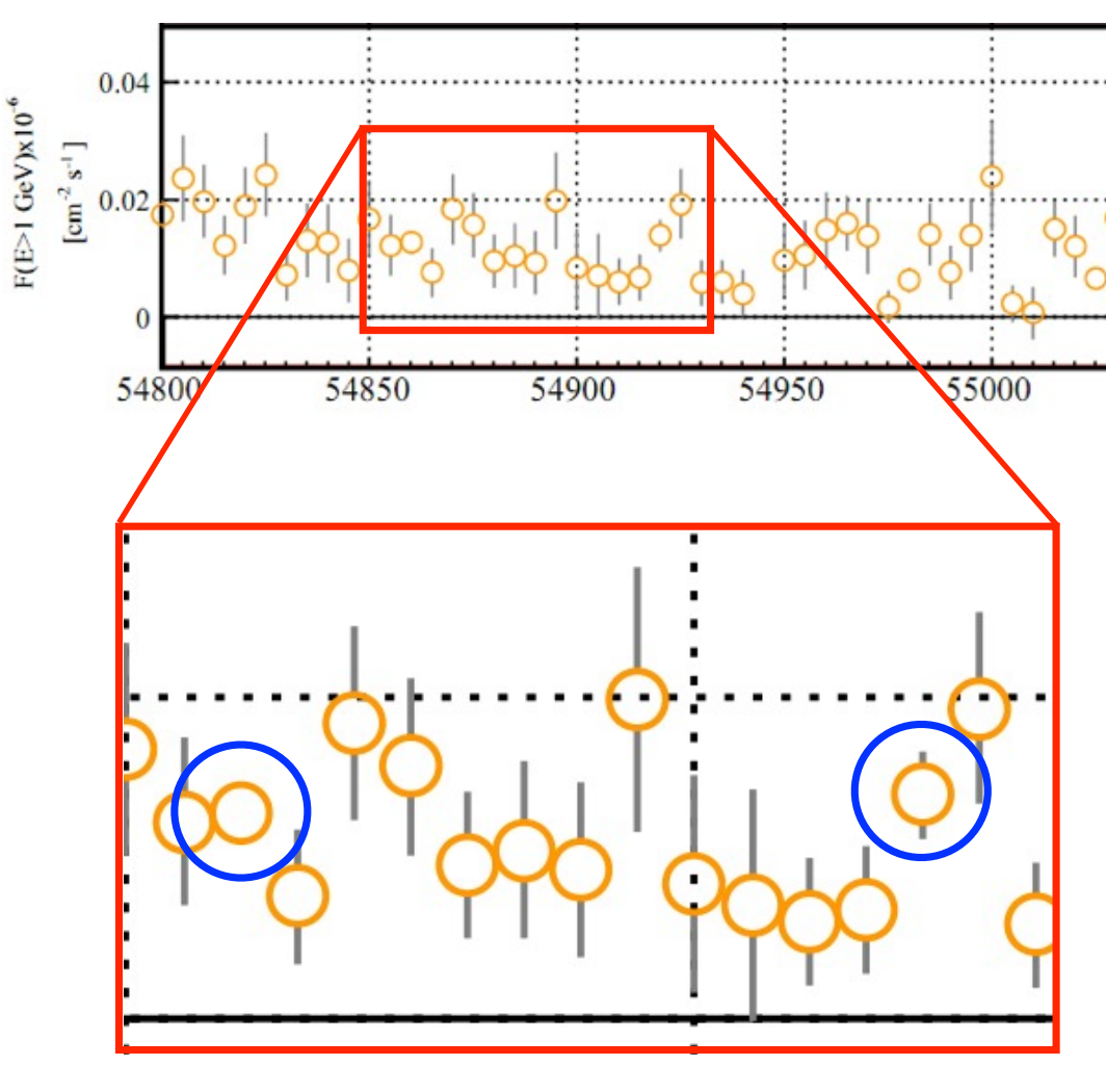
• In this plot, right point has smaller error bar than others at same flux level.
• Left point has error bar so small it is not visible. Potential disaster for variability test.

Automated test?

• Need some automatic way to find points whose errors are “too small”
• Minimum error (variance) is given by Cramer-Rao bound. But that is not calculated in ST.
• Recognize that if source model has converged and predicts $N_{pred}$ counts, then ratio of flux error to flux ($\sigma_F/F$) should not be better than that of Poisson counts underlying measurement: $\sqrt{N_{pred}}/N_{pred}$.

Simple test to find such points

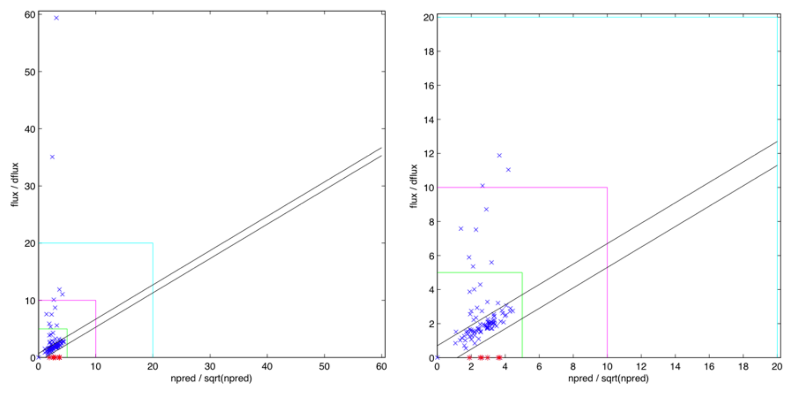
• Plot of $F / F_{err}$ to $N_{pred} / \sqrt{N_{pred}}$ and find outliers. These should be investigated.

from math import *
import BinnedAnalysis
obs = ...
like = ...
like.fit()
src = 'VER0521'
flux = like.normPar(src).getValue()
error = like.normPar(src).error()
N_{pred} = like.N_{pred}Value(src)
print error/flux, sqrt(N_{pred})/N_{pred}
# 0.0281931953422 0.421340108935
print like.optObject.getRetCode()
# 102 --> Anything other than zero indicates problems

Check MINUIT status

gtlike chtter=3 ...:

ERR MATRIX NOT POS-DEF
Minuit fit quality: 2 estimated distance: ...

pyLikelihood:

obs = BinnedObs(...)
like = BinnedAnalysis(obs, 'model.xml', 'MINUIT')
minuit_obj = pyLike.Minuit(like.logLike)
like.fit(covar=True, optObject=minuit_obj)
distance_from_minimum = minuit_obj.getDistance()
qual = minuit_obj.getQuality()

$0$: Error matrix not calculated at all
$1$: Diagonal approximation only, not accurate
$2$: Full matrix, but forced positive-definite (i.e. not accurate)
$3$: Full accurate covariance matrix (After MIGRAD, this is the indication of normal convergence.)

Conjunctions with the Sun

Conjunctions with the Sun can lead to contamination of the LC by gamma rays from the Sun. In 2FGL we flag all periods when the sun-to-source separation is less than 2.5deg.

• Always check the ecliptic coordinates of the source.
• For sources with low ecliptic latitude remove time periods where the source-to-Sun separation is small.

Recommendations for LC

• Follow the strategy of 1FGL / 2FGL.
• Freeze spectral shape parameters ($\Gamma$, $\alpha$/$\beta$, $E_b$, etc).
• Freeze very weak background sources that have very low TS values.
• Set threshold on $TS$, ${\Delta}F/F$ (and $N_{pred}$?) and calculate upper limits for weaker sources.
• Look for suspicious points! Check MINUIT status.

Variability testing

• If you claim variability (or lack of it) then a quantitate test is a good idea.
• Different variability tests are available and may be useful in certain circumstances.
  - 1FGL $\chi^2$ test for a constant flux
  - 2FGL likelihood test for a constant flux
  - Bayesian blocks test for Poisson process
• 2FGL method is more sensitive than 1FGL (but more complex to compute).

1FGL variability index

$\chi^2$ criterion based on best-fit fluxes and flux errors in LC.

Where $f_{rel}$ is the systematic errors.
No variability: $V \sim \chi^2(N-1)$.
Prescription to include upper limits and systematic errors in exposure.

Problems with 1FGL method

• The 1FGL method gives significantly smaller values than expected from $\chi^2$ statistics, therefore is less sensitive to variable sources than desired.
• In this method, likelihood is assumed Gaussian. But not true for weak fluxes.
• In 2FGL variability index is based on actual likelihood.

2FGL variability index

• The 2FGL variability index is based on a comparison of the log-likelihood values for the time bins under two hypothesis:
  - $0$). Null hypothesis: the flux is constant in all time bins - $F_{const}$ - found by ML over all bins.
  - $1$). Alternate hypothesis: the source flux in each bin is different - $F_{i}$ - found by ML in each bin.
• Sum log likelihoods in each - $logL^{(0)}$ & $logL^{(1)}$
• Wilks’ theorem: $TS_{var} = 2{\Delta}L \sim \chi^2(N-1)$
• How to find $F_{const}$? Minimized over all bins?
• Turns out that in mant circumstance $F_{const}$ is close to the value of the source flux from the global analysis - $F_{const} \approx F_{Tot}$
• This was assumed to be true in 2FGL
• This gives a simple recipe - compre the summed likelihood with the flux optimized in each bin to the summed likelihood with $F_{Tot}$
• Can improve on this - e.g. try $F_{Tot}$ & $F_{Tot} \pm x{\Delta}F_{Tot}$

Recipe: 2FGL variability

1. Analysis full time range - global analysis
2. Determine binning
3. Prepare global model
4. Optional: decide criteria for upper limits
   • The 2FGL variability index works whether you calculate ULs or not
5. Divide data into bins
6. Run likelihood analysis on each bin
   a). using global model, but with the flux of the source of interest frozen at its global value. Record total likelihood value - $logL_{i}^{(0)}$
   b). Optional: repeat last step with flux frozen at values of say $F_{Tot} \pm \frac{1}{2}{\Delta}F_{Tot}$ & $F_{Tot} \pm {\Delta}F_{Tot}$ - in this case there are multiple test values of $logL_{i}^{(0)}$ for the different fluxes tried. c). as normal with source flux free - $logL_{i}^{(1)}$
7. Check each analysis for problems
8. Optional: compute upper limits
9. Calculate the summed likelihood under the two hypothesis: $logL^{(0)}$ and $logL^{(1)}$
   • Optional: if multiple test values of $logL^{(0)}$ were calculated (step 6b) then the peak should be found byb fitting a parabola to the three points around the highest
10. Calculate $TS_{var}$

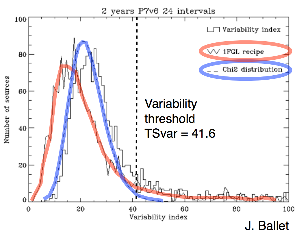
Is 2FGL method better?

Better agreement with $\chi^2$ distribution than 1FGL method. Values slightly larger than expected. But:

• Source variability present to some degree (AGN)
• Small systematic in exposure calculation
• In 2FGL $F_{const}$ was not optimized explicitly

Spectral issues

Spectral model comparisions

• Changed in $2{\Delta}L$ allows “nested” spectral models to be compared statistically - Log-parabola (LP) to power law (PL) - Broken power law (BPL) to PL - PL with exponential cutoff (PLE) to PL
• But be careful comparing non-nested models, e.g. trying to choose between BPL and LP
• Absolute “goodness of fit” measure using flux in band values and $\chi^2$ fit.
  1. Calculate flux in band values
  2. Calculate BPL, LP, PLE model prediction for each band
  3. Compute $\chi^2$ for each model